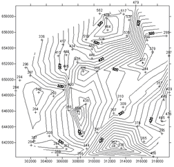
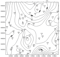
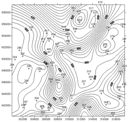
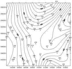
Examples of each of 10 methods for generating the grids described in Table 6‑2 are plotted in Figure 6‑31C‑L. The source data in this case is a set of 62 spot heights from the GB Ordnance Survey NT04 tile, which covers part of the Pentland Hills area to the south of Edinburgh. Also shown is the source OS vector file of contours for this region at 20m contour intervals. Each of the plotted maps has been generated with a 20m contour interval using the methods listed and taking their default parameter settings as provided within the Surfer package.
If the input {x,y,z} dataset is already a complete or nearly complete set of grid values, little or no interpolation is required — simple nearest-neighbor methods are typically used for filling in missing values in such cases.
There are several key points to note about these maps and the data used to generate them:
•all the derived contour maps shown have been generated by first creating a grid file using the interpolation procedure in question, and then contouring applied using linear grid interpolation (as described in the Section 6.5.3, Contouring)
•with a highly variable surface such as this, 62 data points are insufficient to re-create the source data, despite the relatively small size of the region in question
•two of the interpolation methods (natural neighbor and triangulation plus linear interpolation) limit their extent to the convex hull of the input point set
•some methods, including moving averages, nearest-neighbor and triangulation produce very unsatisfactory-looking results with this dataset
•several methods generate very similar looking results, notably natural neighbor and Kriging, and minimum curvature and modified Shepard (see further, Sections 6.6, Deterministic Interpolation Methods, and 6.7, Geostatistical Interpolation Methods)
•interpolation methods based on profiles tend to produce much better results, since these use contour data as their primary input, from which they generate a grid
•interpolation methods based on some arrangements of data points (e.g. points selected along contour lines) can easily result in misleading or erroneous results
Table 6‑2 Gridding and interpolation methods
Method |
Speed |
Type |
Comments |
|---|---|---|---|
Inverse distance weighting (IDW) |
Fast |
Exact, unless smoothing factor specified |
Tends to generate bull’s eye patterns. Simple and effective with dense data. No extrapolation. All interpolated values between data points lie within the range of the data point values and hence may not approximate valleys and peaks well |
Natural neighbor |
Fast |
Exact |
A weighted average of neighboring observations using weights determined by Voronoi polygon concepts. Good for dense datasets. Typically implementations do not provide extrapolation |
Nearest-neighbor |
Fast |
Exact |
Most useful for almost complete datasets (e.g. grids with missing values). Does not provide extrapolation |
Kriging -Geostatistical models (stochastic) |
Slow/ Medium |
Exact if no nugget (assumed measurement error) |
Very flexible range of methods based on modeling variograms. Can provide extrapolation and prediction error estimates. Some controversy over aspects of the statistical modeling and inference. Speed not substantially affected by increasing number of data points. Good results may be achieved with <250 data points |
Conditional simulation |
Slow |
Exact |
Flexible range of techniques that use a fitted variogram as a starting point. Effective as a means of reproducing statistical variation across a surface and obtaining pseudo-confidence intervals |
Radial basis |
Slow/ Medium |
Exact if no smoothing value specified |
Uses a range of kernel functions, similar to variogram models in Kriging. Flexible, similar in results to Kriging but without addition assumptions regarding statistical properties of the input data points |
Modified Shepard |
Fast |
Exact, unless smoothing factor specified |
Similar to inverse distance, modified using local least squares estimation. Generates fewer artifacts and can provide extrapolation |
Triangulation with linear interpolation |
Fast |
Exact |
A Delaunay triangulation based procedure. Requires a medium-large number of data point to generate acceptable results. |
Triangulation with spline interpolation |
Fast |
Exact |
A Delaunay triangulation based procedure, with bicubic spline fitting rather than plane surface fitting. Generates very smooth surfaces. Widely used in computer-aided design |
Profiling |
Fast |
Exact |
A procedure that converts contour data to grid format. Similar to linear interpolation methods used in generating contour data (see subsection 6.5.3, Contouring). See also, subsection 6.6.14, Topogrid/Topo to raster |
Minimum curvature |
Medium |
Exact/Smoothing |
Generates very smooth surfaces that exactly fit the dataset |
Spline functions |
Fast |
Exact (smoothing possible) |
Available as a distinct procedure and incorporated into a number of other methods. Bicubic and biharmonic splines are commonly provided (see for example, Sandwell, 1987) |
Local polynomial |
Fast |
Smoothing |
Most applicable to datasets that are locally smooth |
Polynomial regression |
Fast |
Smoothing |
Provides a trend surface fit to the data points. Most effective for analyzing 1st–order (linear) and 2nd-order (quadratic) patterns, and residuals analysis/trend removal. Can suffer from edge effects, depending on the data. See also, Section 5.6, Spatial Regression |
Moving average |
Fast |
Smoothing |
Uses averages based on a user-defined search ellipse. Requires a medium-large number of data points to generate acceptable results |
Topogrid/Topo to Raster |
Slow/ Medium |
Not specified |
Based on iterative finite difference methods. Interpolates a hydrologically “correct” grid from a set of point, line and polygon data, based on procedures developed by Hutchinson (1988, 1989, 1996). Requires contour vector data as input. Available in ArcGIS based on Hutchinson’s ANUDEM program |
In Figure 6‑31 a series of contour plots are provided, in each case based on the set of GB Ordnance Survey spot heights shown in Figure 6‑31A (Pentland Hills, OS NT04). The first plot, Figure 6‑31B, shows the GB Ordnance Survey contour map for the same region, as a base for comparison purposes. The subsequent contour maps show the results obtained using a variety of interpolation techniques that have been applied to the source spot heights. These are each discussed in more detail in Sections 6.6 and 6.7.
Figure 6‑31-1 Contour plots for alternative interpolation methods — generated with Surfer 8
A. Source data — spot heights, OS NT04
|
B. Source data — contours, OS NT04
|
C. Inverse distance weighting, 1/d2
|
D. Natural neighbor
|

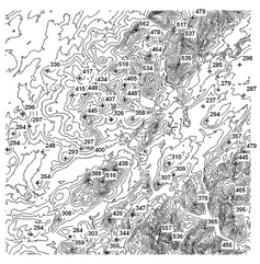
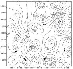
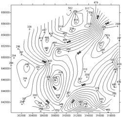
Figure 6‑31-2 Contour plots for alternative interpolation methods — generated with Surfer 8
E. Nearest-neighbor
|
F. Kriging — linear variogram
|
G. Radial basis — quadric function
|
H. Modified Shepard
|
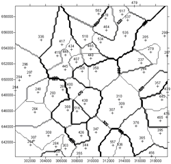
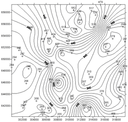
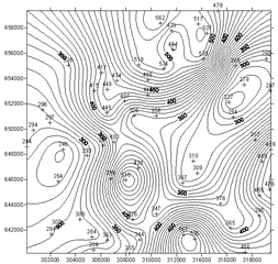
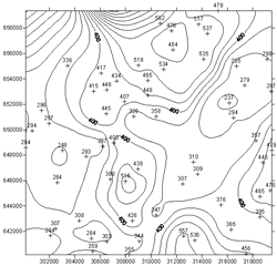
Figure 6‑31-3 Contour plots for alternative interpolation methods — generated with Surfer 8
I. Triangulation with linear interpolation
|
J. Minimum curvature
|
K. Radial basis — bicubic spline, no smoothing
|
L. Local polynomial — linear
|